library(matrixStats)
library(readxl)
library(dplyr)
library(stringr)
library(readr)
library(ggplot2)
library(ggrepel)
library(scales)
library(patchwork)Take_Home_Exercise01
1. Overview
This first take-home project aims to provide a detailed visualization of Singapore’s demographic structure in 2024. Three visual representations will be described and implemented in this project:
A population pyramid shows age-sex bulges, gaps, and the median age.
A bar-chart comparison tries to compare population distribution between young and old groups.
A bubble scatter which maps youth vs. elderly shares, with bubble size for population and color for median age.
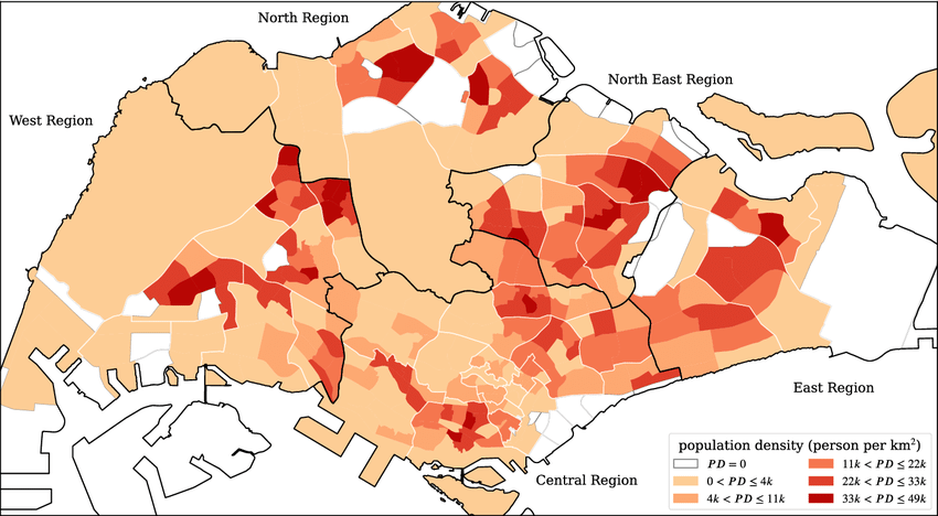
Before we go deeper into analysis, a simple map can give us a great overview of population density of Singapore, the lighter color indicates a lower population density, which is mainly concentrated in the West and central region, while the darker color marks zones with a higher density, which are mainly in the East Region and central part of the country. Through this project we aim to provide useful information of Singapore’s population distribution and to understand the eventual divergence between different gender and/or age groups.
Note
Source: Spatial super-spreaders and super-susceptibles in human movement networks - Scientific Figure on ResearchGate. Available from: https://www.researchgate.net/figure/The-subzone-residential-population-density-map-of-Singapore-PD-stands-for-population_fig1_346481200 [accessed 1 May 2025]
1.1 Setting the scene
A local online media company that publishes daily content on digital platforms is planning to release an article on demographic structures and distribution of Singapore in 2024.
The goal is to transfer useful demographic information to the audience by providing some visual graphics that answer questions such as:
“Where do the youngest and oldest residents live?”
“How balanced is country’s working-age population?”
“Are Singaporean birthrates falling?”
…
By setting these hypothetical question, we are not only providing a data visualization project, but also aiming to meet some real business needs and contribute to possible accademic research.
1.2. Data structure
The dataset is Singapore Residents by Planning Area / Subzone, Single Year of Age and Sex, June 2024, which is from the Department of Statistics (DOS). In total, after expanding 55 planning areas and roughly 323 subzones, across 92 age bins (Under 1, 1–89, and “90 and over”), and two sexes, the raw file runs to about 32 000 rows. Here is a summary of data structure:
| Column | Type | Description | Example |
|---|---|---|---|
| Planning Area | Text | One of the 55 official planning areas designated by URA. | Central Area |
| Subzone | Text | A finer subdivision within each planning area | Chinatown |
| Age | Text | Single-year age categories plus special labels for youngest (“Under 1”) and oldest (“65 and over”, “90 and over”). | Under 1; 27; 65 and over |
| Sex | Text | Resident gender | Female |
| Population | Text→Numeric | Resident count for June 2024. Imported as text (formatting) then cast to numeric for analysis. | “10356” → 10356 |
2. Data cleaning
2.1 Load the necessary packages
Before starting the analysis, we install and load a set of R packages that help our data‐wrangling, text-parsing, and visualization toolkit:
| Package | Description |
|---|---|
| matrixStats | Provides optimized, vectorized functions for row‐ and column‐wise summaries on matrices. |
| readxl | Used to import Excel files (.xls and .xlsx) into R data frames without requiring Java or external dependencies. |
| dplyr | A grammar of data manipulation. |
| stringr | A consistent wrapper around R’s string‐processing functions, built on the {stringi} engine. |
| readr | Provides functions for reading flat files (CSV, TSV, FWf). |
| ggplot2 | Implements the “Grammar of Graphics” for creating complex, multi‐layered visualizations. |
| ggrepel | An add‐on to ggplot2 that smartly repels text and label annotations so they do not overlap. |
| scales | Provides a suite of functions for transforming and formatting axis breaks, labels, and legends. |
| patchwork | Used for assembling multiple ggplot2 plots into complex layouts without resorting to low‐level grid hacks. |
2.2 Data cleaning
The data is loaded into environment by eliminating those rows with values “Total” for the reason that it could construct a distortion of data analysis at individual-area or individual-age level. The imported data (column: ‘Population’) has been converted into numeric format that ensures the future algebraic calculation (sum, average, or counts).
Many values of column ‘Age’ has been transformed:
“Under x” entries (e.g. “Under 1”) become age 0.
“Over x” or “x and over” (e.g. “65 and over”) are parsed to the base number (65).
Any rows where the population or parsed age turned into null values are removed. This guards against stray text labels or malformed entries that slipped past the earlier filters.
# 1. Read in data and drop all “Total” summary rows
df_clean <- read_excel("respopagesex2024e.xlsx") %>%
  filter(
    `Planning Area` != "Total",
    Subzone         != "Total",
    Sex             != "Total"
  ) %>%

  # 2. Convert population to numeric
  mutate(
    Population = as.numeric(`2024`),

    # 3. Parse Age into a single-year numeric
    Age_numeric = case_when(
      str_detect(Age, regex("under",    ignore_case = TRUE)) ~ 0,
      str_detect(Age, regex("over|and over", ignore_case = TRUE)) ~ parse_number(Age),
      TRUE ~ as.numeric(Age)
    )
  ) %>%

  # 4. Remove any rows that failed conversion
  filter(
    !is.na(Population),
    !is.na(Age_numeric)
  )
After the data cleaning process, we display some rows to check:
# 5. Inspect
glimpse(df_clean)
Rows: 37,243
Columns: 7
$ `Planning Area` <chr> "Ang Mo Kio", "Ang Mo Kio", "Ang Mo Kio", "Ang Mo Kio"…
$ Subzone <chr> "Ang Mo Kio Town Centre", "Ang Mo Kio Town Centre", "A…
$ Age <chr> "0", "0", "1", "1", "2", "2", "3", "3", "4", "4", "5",…
$ Sex <chr> "Males", "Females", "Males", "Females", "Males", "Fema…
$ `2024` <chr> "10", "10", "10", "10", "10", "10", "10", "10", "30", …
$ Population <dbl> 10, 10, 10, 10, 10, 10, 10, 10, 30, 10, 20, 10, 20, 30…
$ Age_numeric <dbl> 0, 0, 1, 1, 2, 2, 3, 3, 4, 4, 5, 5, 6, 6, 7, 7, 8, 8, …head(df_clean, 10)# A tibble: 10 × 7
`Planning Area` Subzone Age Sex `2024` Population Age_numeric
<chr> <chr> <chr> <chr> <chr> <dbl> <dbl>
1 Ang Mo Kio Ang Mo Kio Town Ce… 0 Males 10 10 0
2 Ang Mo Kio Ang Mo Kio Town Ce… 0 Fema… 10 10 0
3 Ang Mo Kio Ang Mo Kio Town Ce… 1 Males 10 10 1
4 Ang Mo Kio Ang Mo Kio Town Ce… 1 Fema… 10 10 1
5 Ang Mo Kio Ang Mo Kio Town Ce… 2 Males 10 10 2
6 Ang Mo Kio Ang Mo Kio Town Ce… 2 Fema… 10 10 2
7 Ang Mo Kio Ang Mo Kio Town Ce… 3 Males 10 10 3
8 Ang Mo Kio Ang Mo Kio Town Ce… 3 Fema… 10 10 3
9 Ang Mo Kio Ang Mo Kio Town Ce… 4 Males 30 30 4
10 Ang Mo Kio Ang Mo Kio Town Ce… 4 Fema… 10 10 43 Objective and research question definition
One of the purpose of data visualization project is to answer specific research question, here we are proposing many possible research question that could be useful in term of demographic analysis of Singapore population.
3.1 National Age–Sex Structure for 2024
The gender is the key attribute in most of demographic analysis, by focusing on this element, we are trying to formulate the following research questions:
What is the male and female age distribution in 2024?
Which male and/or female age groups show unusual trends and what is possible reason of that?
Are there gender-specific patterns?
Analytical Approach:
Aggregate cleaned dataset by Age_numeric and Gender to compute total residents.
Transform these into within-sex percentage shares.
Identify Extremes: compute weighted median age; select top 3 bulge cohorts
Visualize with ggplot2: geom_col() for the back-to-back bars; geom_vline() + annotate() for median age; geom_segment() + geom_text() arrows for bulges; geom_point() + labels for gaps; coord_flip(), absolute y-axis labels, and a clean theme.
3.3 Spatial Patterns: Median Age & Population Density
A more complex analysis can be done by combining population age and density, here we are trying to answer these questions:
How do youth and elderly shares co-vary across all 55 planning areas?
Are “youth hubs” (high under-15 & high density) distinct from “retirement clusters” (high 65+ & low density)?
What role does median age play in these groupings?
Analytical Approach:
Compute Metrics for each Planning Area: youth_share, elderly_share, total_pop = sum(Population), median_age = weightedMedian(Age_numeric, Population)
Global Benchmarks: calculate means and Pearson r.
Plot with ggplot2: aes(x = youth_share, y = elderly_share, size = total_pop, color = median_age); geom_point() + geom_smooth(method=“lm”, linetype=“dotted”); geom_vline()/geom_hline() at mean shares; ggrepel::geom_text_repel() to label areas; Color scale (viridis_c()), percent axes, and a minimal theme.
3.4 Visualization Deliverables
| deliverable | Research Question(s) | Plot Type | Key Features |
|---|---|---|---|
| 1. Population Pyramid | 3.1 What does Singapore’s age–sex profile look like in 2024? | Back-to-back bar chart (geom_col) |
Males left/females right; weighted median line |
| 2. Top-10 Youth vs. Elderly Bar Charts | 3.2 Which planning areas have the highest share under 15? Which have the highest share 65 +? | Horizontal bar charts (geom_col) |
Green bars for under 15; red bars for 65 +; top 10 lists; percent-formatted x-axis; patchwork layout |
| 3. Youth-Elderly Bubble Scatter | 3.3 How do youth and elderly shares co-vary across all planning areas? What role does median age play? | Scatter plot with bubbles (geom_point) |
x = share < 15; y = share ≥ 65; bubble size = total pop; color = median age; regression line + labels |
4 Visualization elaboration
4.1 Visualization 1 (National Age–Sex Structure for 2024)
To create the pyramid graph, we assign the clean dataset to ‘pyramid_df’ and group the data by ‘Sex’ and ‘Age_numeric’, and for each (Sex,Age_numeric) group, we count the total resident. By using ‘mutate’ function, we are going to transform raw counts into per-sex percentages, then turns the result into signed and absolute forms for plotting and annotation.
# 1. Build pyramid_df with percentage shares
pyramid_df <- df_clean %>%
  group_by(Sex, Age_numeric) %>%
  summarise(Pop = sum(Population, na.rm=TRUE), .groups="drop") %>%
  group_by(Sex) %>%
  mutate(
    PopPct    = Pop / sum(Pop),
    PopSigned = if_else(Sex=="Male", -PopPct, PopPct),
    PopAbs    = abs(PopSigned)
  ) %>%
  ungroup()
We compute also weighted median age by using function ‘weightedMedian’:
# 2. Compute weighted median age
med_age <- weightedMedian(df_clean$Age_numeric, w=df_clean$Population)
Through ggplot function, we generated the pyramide plot:
# 4. Plot as percent pyramid with annotations
ggplot(pyramid_df, aes(x=Age_numeric, y=PopSigned, fill=Sex)) +
  geom_col(width=1, color="white") +

  # median‐age line
  geom_vline(xintercept=med_age, linetype="dashed", color="grey40") +
  annotate("text",
           x = med_age + 2, y = 0,
           label = paste0("Median age: ", med_age),
           angle=90, vjust=-0.5, size=3) +

  # percent scales & flip
  scale_y_continuous(labels=percent_format(accuracy=1)) +
  coord_flip() +
  scale_fill_brewer(palette="Set2") +

  # labels & theme
  labs(
    title    = "Singapore Population Pyramid (2024)",
    subtitle = "Cohort % shares; median & peaks/gaps annotated",
    x        = "Age (years)",
    y        = "% of sex population",
    fill     = NULL
  ) +
  theme_minimal(base_size=12) +
  theme(
    legend.position    = "top",
    panel.grid.major.y = element_blank()
  )
Note
Plot description:
In 2024, Singapore population shows a kind of “double-bulge” pattern and an overall shift toward an older age group. The median age is 42 and top 3 largest age groups are around 33,35, and 36.
Sex differences are also evident: although there is not huge differences between them, the female bars extend further at ages 70+, indicating a higher female longevity. Both gender distributions converge between ages 20–40, that confirms a balanced labor-force cohorts. The chart inspires Singapore’s transition to an older population (as happen in Japan), with age groups “bulges” at 35 and 55, and flags a shrinking base of young children.
4.2 Visualization 2 (Age Distributions by Planning Area)
As mentioned in the analytical approch (3.2 Comparing Youth vs. Elderly Shares), in this phase, we compute the ‘youth_share’ and ‘elederly_share’ by using these formulas:
youth_share = sum(Population[Age_numeric < 15]) / sum(Population)
elderly_share = sum(Population[Age_numeric >= 65]) / sum(Population)
# 1. Compute shares by Planning Area
dep_pa <- df_clean %>%
  group_by(`Planning Area`) %>%
  summarise(
    youth_share   = sum(Population[Age_numeric < 15], na.rm=TRUE) / sum(Population),
    elderly_share = sum(Population[Age_numeric >= 65], na.rm=TRUE) / sum(Population),
    .groups = "drop"
  )
The we display plots for each share group, and put them together:
# 2a. Top 10 youngest areas (highest youth_share)
p_young_pa <- dep_pa %>%
  slice_max(youth_share, n = 10) %>%
  mutate(`Planning Area` = reorder(`Planning Area`, youth_share)) %>%
  ggplot(aes(y = `Planning Area`, x = youth_share)) +
    geom_col(fill = "#2ca25f") +
    scale_x_continuous(labels = percent_format(1)) +
    labs(
      title = "Top 10 Youngest Planning Areas",
      x     = "Share under 15",
      y     = NULL
    ) +
    theme_minimal(base_size = 11)

# 2b. Top 10 oldest areas (highest elderly_share)
p_old_pa <- dep_pa %>%
  slice_max(elderly_share, n = 10) %>%
  mutate(`Planning Area` = reorder(`Planning Area`, elderly_share)) %>%
  ggplot(aes(y = `Planning Area`, x = elderly_share)) +
    geom_col(fill = "#de2d26") +
    scale_x_continuous(labels = percent_format(1)) +
    labs(
      title = "Top 10 Oldest Planning Areas",
      x     = "Share 65 and over",
      y     = NULL
    ) +
    theme_minimal(base_size = 11)

# 3. Display side by side
p_young_pa + p_old_pa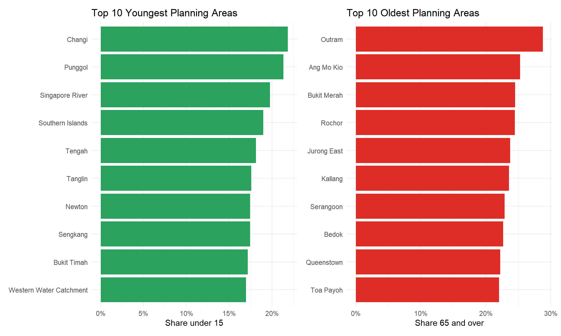
Note
Plot description:
The first plot identifies Changi and Punggol as the “youngest” area of Singapore in 2024, with over 22 % of residents under 15, followed by Singapore River. Southern Islands and Western Water Catchment show high youth shares as well, indicating small but family-oriented populations in those zones. The second plot identifies Outram as the “oldest” district at nearly 29 % of 65 + age group, followed by Ang Mo Kio and Bukit Merah. These mature, inner-city precincts have proportionally more seniors. Areas like Bedok, Queenstown, and Toa Payoh likewise appear, underscoring how Singapore’s first-generation housing towns still house an aging cohort.
The plot contributes to where childhood services (schools, playgrounds) might be most needed (Punggol, Changi, Tengah) and where eldercare resources (community centers, healthcare) should be prioritized (Outram, Ang Mo Kio, Bukit Merah).
4.3 Visualization 3 (Spatial Patterns: Median Age & Population Density)
As done in the previous plot, we have to compute the key metrics for our visualization task by using these formulas:
youth_share = sum(Population[Age_numeric < 15]) / sum(Population)
elderly_share = sum(Population[Age_numeric >= 65]) / sum(Population)
total_pop = sum(Population)
median_age = matrixStats::weightedMedian(Age_numeric, w = Population)
# 1. Compute metrics
dep_shares <- df_clean %>%
  group_by(`Planning Area`) %>%
  summarise(
    youth_share   = sum(Population[Age_numeric < 15], na.rm=TRUE) / sum(Population),
    elderly_share = sum(Population[Age_numeric >= 65], na.rm=TRUE) / sum(Population),
    total_pop     = sum(Population),
    median_age    = matrixStats::weightedMedian(Age_numeric, w = Population),
    .groups       = "drop"
  )
The we compute the average proportion of residents under 15 and over 65 across the 55 planning areas, and the Pearson correlation between each area’s youth share and elderly share.
# 2. National means & correlation
mean_youth   <- mean(dep_shares$youth_share)
mean_elderly <- mean(dep_shares$elderly_share)
corr_val     <- cor(dep_shares$youth_share, dep_shares$elderly_share)
The final plot is the following:
# 2. National means & correlation
mean_youth   <- mean(dep_shares$youth_share)
mean_elderly <- mean(dep_shares$elderly_share)
corr_val     <- cor(dep_shares$youth_share, dep_shares$elderly_share)

# 3. Plot
ggplot(dep_shares, aes(
    x = youth_share,
    y = elderly_share,
    size  = total_pop,
    color = median_age
  )) +
  geom_smooth(method = "lm", se = FALSE, color = "grey40", linetype = "dotted") +
  geom_vline(xintercept = mean_youth,   linetype = "dashed", color = "grey60") +
  geom_hline(yintercept = mean_elderly, linetype = "dashed", color = "grey60") +
  geom_point(alpha = 0.8) +
  geom_text_repel(
    aes(label = `Planning Area`),
    size       = 3,
    max.overlaps = 20
  ) +
  scale_x_continuous(labels = percent_format(1)) +
  scale_y_continuous(labels = percent_format(1)) +
  scale_size(range = c(2, 10), labels = comma_format(accuracy = 1), name = "Total pop") +
  scale_color_viridis_c(option = "magma", name = "Median age") +
  annotate(
    "text",
    x    = 0.30,
    y    = 0.20,
    label= paste0("r = ", round(corr_val, 2)),
    size = 4,
    color= "black"
  ) +
  labs(
    title    = "Youth vs. Elderly Shares by Planning Area",
    subtitle = "Bubble size ~ total population; Color ~ median age",
    x        = "Share of residents under 15",
    y        = "Share of residents 65 and over"
  ) +
  theme_minimal(base_size = 12) +
  theme(
    legend.position = "right",
    panel.grid.minor = element_blank()
  )
Note
Plot description:
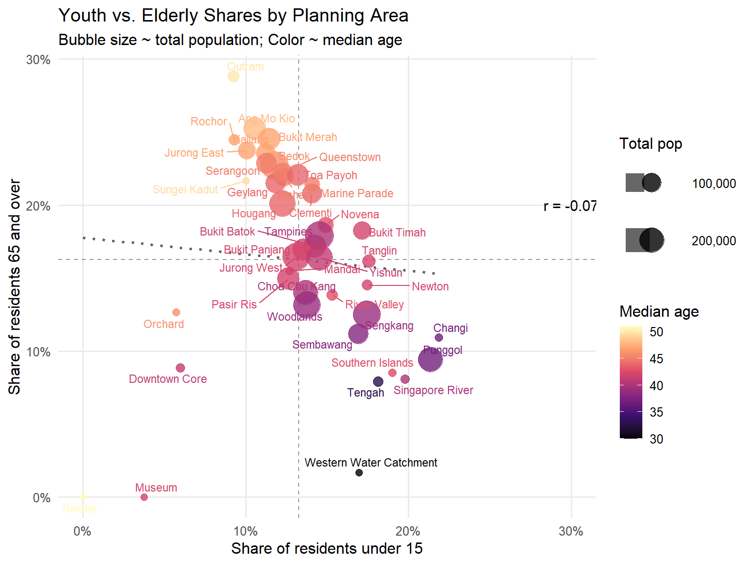
On the x-axis (‘Shares of residents under 15’), Punggol, Changi, and Southern Islands lie far right as confirmed in the visualization 2, indicating 20–30 % of residents under 15. On the y-axis (‘Share of residents 65 and over’), Outram, Rochor, and Ang Mo Kio sit near 25–30 % aged 65 +, marking them as “retirement clusters.” The vertical and horizontal dashed lines show national average shares (~13 % youth, ~17 % elderly), and the dotted regression line (r ≈ –0.07) confirms almost no linear trade-off between youth and senior population, means that changes in youth shares do not reliably predict changes in elderly shares.
Punggol’s large dot highlights its sizable young population, while Outram has a small portion of residents but the highest percentage of “retirement clusters”. This visualization indicates true “youth hubs” and “elder hubs” at a glance, enriched by population and age-structure context.
4.4 Conclusion
The pyramid plot shows that Singapore’s population reveals a clear shift toward an older population, and a higher longevity of female resident compared to male groups. By examining the planning ares data, Changi and Punggol are unmistakable “youth hubs” (as confirmed in visualization 2,3), whereas Outram, Ang Mo Kio and Bugit Merah stand out as “retirement clusters”.
An interesting part is shown in the visualization 3, which confirms that extreme concentrations of children and seniors seldom overlap and most districts clustering near the national average. Likewise, the correlation indicator (r = -0.07) indicates there is no significant correlation between two groups, changes in youth shares will not affect elderly population. Most of area are in the middle position rather than being an outlier of the data.